Lecture notes. Written from the material of Berkeley Stat 153, licensed CC BY 4.0. These are notes, not a transcript: the material has been reorganised and rewritten. This adaptation carries the same licence, and the original is linked above.

3. Autocovariance and Stationarity

What this covers

This chapter answers two connected questions. First, given a time series (or a pair of them), how do you measure the dependence between its values at different times — the autocovariance, autocorrelation, cross-covariance and cross-correlation? Second, when is that dependence structure stable enough over time that it can actually be estimated from a single observed run — the idea of stationarity, and why weak stationarity rather than the strict version is the working definition. It assumes the basic time series vocabulary from earlier lectures: white noise, moving averages, random walks with drift, and ordinary covariance and variance.

Covariance of linear combinations

The tool underneath everything below is bilinearity of covariance. If \(U = \sum_{j=1}^m a_j X_j\) and \(V = \sum_{k=1}^r b_k Y_k\) are linear combinations of finite-variance random variables \(X_j\) and \(Y_k\), then

\[\operatorname{cov}(U,V) = \sum_{j=1}^m \sum_{k=1}^r a_j b_k \, \operatorname{cov}(X_j, Y_k).\]

Covariance of a sum is the sum of the pairwise covariances, weighted by the coefficients. This is exactly what is needed once a time series is written as a linear combination of simpler pieces — as a random walk is.

The autocovariance function

For a single time series \(x_t\), define the autocovariance function

\[\gamma(s,t) = \operatorname{cov}(x_s, x_t).\]

Worked example: the random walk. Recall the random walk with drift, \(x_t = \delta t + \sum_{i=1}^t w_i\), where the increments \(w_i\) are uncorrelated (variance \(\sigma^2\) each, mean zero). To find \(\gamma(s,t)\), write both \(x_s\) and \(x_t\) as sums and apply bilinearity. The drift terms \(\delta s\) and \(\delta t\) are constants, so they drop out of any covariance. What is left is

\[\gamma(s,t) = \operatorname{cov}\!\left(\sum_{i=1}^s w_i,\; \sum_{j=1}^t w_j\right) = \sum_{i=1}^s\sum_{j=1}^t \operatorname{cov}(w_i,w_j).\]

Because the \(w_i\) are uncorrelated, every cross term with \(i \neq j\) vanishes, and only the terms with \(i=j\) survive, each contributing \(\operatorname{Var}(w_i) = \sigma^2\). The number of indices common to both sums is \(\min(s,t)\), so

\[\gamma(s,t) = \sigma^2 \min(s,t).\]

This is worth pausing on: the answer depends on the actual times \(s\) and \(t\), not just on how far apart they are. \(\gamma(1,2) = \sigma^2\) but \(\gamma(100,101) = 100\sigma^2\) — two pairs of observations one step apart, with wildly different covariance depending on when they occur. That is the property that will disqualify the random walk from being stationary below.

The autocorrelation function

Raw covariance is unbounded and depends on the scale of the series, so it is useful to normalize it. The autocorrelation function (ACF) is

\[\rho(s,t) = \frac{\gamma(s,t)}{\sqrt{\gamma(s,s)\,\gamma(t,t)}}.\]

This measures the linear predictability of \(x_t\) from \(x_s\): how well a linear function of \(x_s\) predicts \(x_t\). Because \(\gamma(s,s) = \operatorname{Var}(x_s)\) and \(\gamma(t,t) = \operatorname{Var}(x_t)\), the Cauchy–Schwarz inequality for covariance,

\[|\operatorname{cov}(x,y)| \leq \sqrt{\operatorname{Var}(x)\operatorname{Var}(y)},\]

guarantees \(-1 \leq \rho(s,t) \leq 1\), with the endpoints reached exactly when \(x_t\) is an exact increasing or decreasing linear function of \(x_s\).

Cross-covariance and cross-correlation

The same idea extends to comparing two different time series, \(x_t\) and \(y_t\). The cross-covariance function is

\[\gamma_{xy}(s,t) = \operatorname{cov}(x_s,y_t) = \mathbb{E}[(x_s-\mu_{xs})(y_t-\mu_{yt})],\]

and it captures how the values of \(y\) at time \(t\) relate to the values of \(x\) at time \(s\).

Worked example. Take the simplest possible relationship: \(y_t = x_{t-2}\), so \(y\) is literally a copy of \(x\) delayed by two steps. What does \(\gamma_{xy}\) look like, and at which lag is it largest? Substituting directly,

\[\gamma_{xy}(s,t) = \operatorname{cov}(x_s, x_{t-2}) = \gamma_x(s,\,t-2),\]

so the cross-covariance between \(x\) and \(y\) is just the autocovariance of \(x\) itself, evaluated between \(s\) and \(t-2\) instead of between \(s\) and \(t\). Writing the gap as \(h = s-t\), this is \(\gamma_x(h+2)\) in terms of \(x\)'s own lag. By the same Cauchy–Schwarz bound used for the ACF, \(|\gamma_x(\cdot)|\) is largest when its two time arguments coincide — i.e. at lag \(0\) — so \(\gamma_{xy}(h) = \gamma_x(h+2)\) is largest at \(h = -2\). That matches the intuition directly: \(y_t\) is \(x_{t-2}\), so the strongest link between the two series shows up exactly when you shift \(x\) back two steps to line it up with \(y\).

The normalized version is the cross-correlation function,

\[\rho_{xy}(s,t) = \frac{\gamma_{xy}(s,t)}{\sqrt{\gamma_x(s,s)\,\gamma_y(t,t)}},\]

again bounded between \(-1\) and \(1\) by the same argument.

Stationarity

All of the definitions above allow the dependence structure to change arbitrarily with time, as the random walk example just showed. That is a problem for estimation: with a single observed run of a time series, there is only one realization of \(x_s\) and one of \(x_t\) for each pair, so nothing about \(\gamma(s,t)\) can be estimated unless the dependence structure repeats itself across time in some way.

A time series \(x_t\) is strictly stationary if every finite collection of its values has the same joint distribution as the same collection shifted forward in time:

\[\{x_{t_1}, x_{t_2}, \dots, x_{t_k}\} \overset{d}{=} \{x_{t_1+h}, x_{t_2+h}, \dots, x_{t_k+h}\}\]

for every \(h\) and every choice of times — meaning identical means, variances, and all higher-order moments, for all \(t\). An i.i.d. process is the standard example. This is too strong a requirement for most applications, so the working definition used going forward is weaker.

A time series \(x_t\) (with finite variance) is weakly stationary if:

• its mean function is constant, not depending on \(t\): \(\mu_t = \mu\);
• its autocovariance function \(\gamma(s,t)\) depends on \(s\) and \(t\) only through the difference \(|s-t|\).

Writing \(s = t+h\) so that \(h\) is the lag between the two times,

\[\gamma(t+h,t) = \operatorname{cov}(x_{t+h},x_t) = \operatorname{cov}(x_h,x_0) = \gamma(h,0) = \gamma(h),\]

so for a weakly stationary series the autocovariance collapses to a function of a single argument, the lag:

\[\gamma(h) = \operatorname{cov}(x_{t+h}, x_t) = \mathbb{E}[(x_{t+h}-\mu)(x_t-\mu)].\]

(The book being used for this course calls this simply "stationary," as shorthand for weak stationarity.)

The random walk computed above is the concrete illustration of failing this: \(\gamma(s,t) = \sigma^2\min(s,t)\) does not reduce to a function of \(s-t\) alone, so a random walk is not stationary, regardless of what happens with the mean. The general pattern to check going forward: if the mean and/or the autocovariance change with time, the series is not stationary. White noise is strictly stationary, a moving average is (in general) weakly stationary, and both a random walk and a series with a linear trend are not stationary.

Estimating covariance from a single series

The reason stationarity matters practically: most of the time there is only one observed run of the time series, not repeated independent copies at each time \(t\), so \(\mu_t\) cannot be estimated separately for every \(t\). Assuming stationarity collapses the unknown mean to a single constant \(\mu\), which can be estimated by the ordinary sample mean \(\bar{x} = \frac{1}{n}\sum_{t=1}^n x_t\) computed by averaging across time within the one run. The autocovariance is then estimated by

\[\hat{\gamma}(h) = \frac{1}{n}\sum_{t=1}^{n-h}(x_{t+h}-\bar{x})(x_t-\bar{x}), \qquad h = 0,1,\dots,n-1,\]

with \(\hat{\gamma}(-h) = \hat{\gamma}(h)\). This can always be computed from data, whether or not stationarity actually holds — but it is only interpretable as an estimate of a real underlying autocovariance to the extent that the stationarity assumption is approximately true.

The analogous estimator for the relationship between two jointly weakly stationary series \(x_t\) and \(y_t\) is the sample cross-correlation,

\[\hat{\rho}_{xy}(h) = \frac{\hat{\gamma}_{xy}(h)}{\sqrt{\hat{\gamma}_x(0)\,\hat{\gamma}_y(0)}}.\]

The lecture illustrated this with the Southern Oscillation Index (SOI) and a fish recruitment series: the sample ACF of each series individually, and the sample cross-correlation function between them, showing at which lags the two series are most strongly linked — the same question answered above symbolically for \(y_t = x_{t-2}\), now asked of real data.

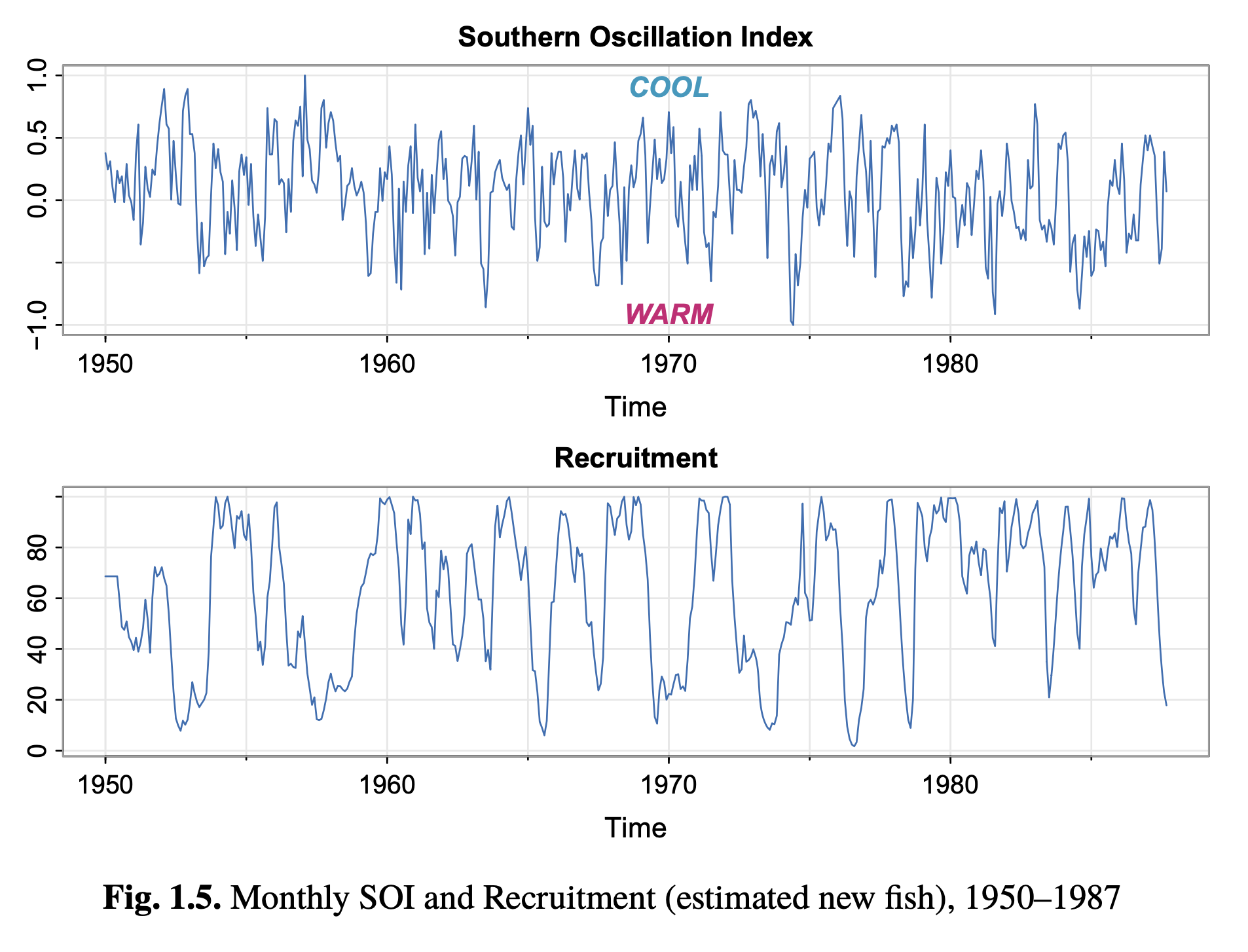
The two raw series: the Southern Oscillation Index and fish recruitment over time.

Sample ACFs of each series and their sample cross-correlation function, showing the lags at which the two series are most related.

Sources

• Slide notes "Today" (Berkeley STAT 153, spring 2026, lecture 4 notes, part 1): covariance of linear combinations, the random walk autocovariance example, the autocorrelation function, cross-covariance and cross-correlation, and the \(y_t = x_{t-2}\) worked example.
• Slide notes "Stationarity" (same lecture, part 2): strict vs. weak stationarity, the lag notation \(\gamma(h)\), the sample autocovariance and sample cross-correlation estimators, and the SOI/fish recruitment figures.
• No transcript, written notes, or problem set were supplied for this lecture; nothing from those sources appears here.
• The lecture's own assigned reading is Shumway and Stoffer, Time Series Analysis, Chapter 1.3–1.7, which the slides summarize but do not reproduce in full — consult it directly for anything not covered above.
• The lecture also referenced an upcoming lab comparing stationarity of white noise, a moving average, a random walk, and a linear trend, and previewed that the next lecture moves to linear regression (Shumway and Stoffer, Chapter 2) — neither the lab nor that material is contained in the supplied slides.

---

← 2. Mean, Autocovariance, and Correlation · Contents · 4. Linear Regression for Time Series →