Lecture notes. Written from the material of Berkeley Stat 153, licensed CC BY 4.0. These are notes, not a transcript: the material has been reorganised and rewritten. This adaptation carries the same licence, and the original is linked above.

16. Identifying ARMA Models via ACF/PACF

What this covers

The previous lecture established that a causal ARMA(p,q) process is stationary. This one asks the practical follow-up: given a real series, how do you tell what \(p\) and \(q\) should be? The answer is a pair of diagnostics, the autocorrelation function (ACF) and the partial autocorrelation function (PACF), read together — and the chapter works through what that pair actually looks like against three real series from the lecture's own notebook. It assumes the ARMA model, causality, invertibility, and the plain ACF are already familiar from the previous lecture.

The ARMA model, briefly recalled

An ARMA(p,q) process is

\[x_t = \sum_{j=1}^p \phi_j x_{t-j} + \sum_{j=0}^q \theta_j w_{t-j},\]

where \(w_t\) is white noise, the coefficients \(\phi_1,\dots,\phi_p,\theta_0,\dots,\theta_q\) are fixed (non-random), \(\phi_p,\theta_q \neq 0\), and \(\theta_0 = 1\) by convention.

Two facts from the previous lecture are used here without re-proving them (the arguments are in Shumway & Stoffer, Appendix B2 and Chapter 3):

• Causality: a causal AR(p) process can be written as an MA(\(\infty\)) process, \(x_t = \sum_{j=0}^\infty \psi_j w_{t-j}\) with \(\sum_{j=0}^\infty |\psi_j| < \infty\).
• Invertibility: an invertible MA(q) process can be written as an AR(\(\infty\)) process, \(x_t = -\sum_{j=1}^\infty \phi_j x_{t-j} + w_t\).

Causality implies stationarity, so an ARMA(p,q) process is stationary exactly when the roots of the \(\phi\) polynomial and the \(\theta\) polynomial lie outside the unit circle. The modelling target is a causal, invertible ARMA fit of the right order — and "the right order" is what the rest of this chapter is about finding.

Why the ACF alone isn't enough

The two building blocks behave very differently in their autocovariance:

• An AR(1) process has autocovariance that decays smoothly away from \(h=0\) and never hits zero exactly.
• An MA(q) process has autocovariance that is exactly zero once \(|h| > q\): the moving average only remembers \(q\) lags back, and there is nothing left to correlate beyond that.

So an MA order should be readable straight off where the ACF hits zero. An AR order is not, because the ACF measures the total correlation between \(x_t\) and \(x_{t-h}\), including correlation transmitted through the lags in between. In an AR(1) process, \(x_t\) and \(x_{t-2}\) are correlated — but only because both are correlated with \(x_{t-1}\); there is no direct dependence at lag 2 at all. The ACF at lag 2 is nonzero regardless.

The ACF at lag 2 includes correlation transmitted indirectly through the intervening lag; the PACF strips that path out by regressing out x(t-1) first.

The partial autocorrelation function

The PACF, written \(\phi_{hh}\), is the correlation between \(x_t\) and \(x_{t-h}\) after regressing out \(x_{t-1}, \dots, x_{t-h+1}\) — the lags strictly between them. It answers a sharper question than the ACF does: does lag \(h\) carry any additional predictive information once you already have lags \(1\) through \(h-1\)?

More generally, for random variables \(X, Y\) and a conditioning set \(Z=\{Z_1,\dots,Z_k\}\), the partial correlation of \(X\) and \(Y\) given \(Z\) is built by regressing each of \(X\) and \(Y\) on \(Z\) separately, then correlating what is left over:

\[\rho_{XY \mid Z} = \mathrm{corr}(X-\hat X,\ Y-\hat Y),\]

where \(\hat X\) and \(\hat Y\) are the fitted values from regressing \(X\) and \(Y\) on \(Z\). (Shumway & Stoffer §3.3.2 works through the derivation of the PACF in the ARMA case in full.)

Because an AR(p) process has no direct dependence beyond lag \(p\), its PACF cuts off cleanly after lag \(p\) — the AR-order analogue of what the ACF does for MA order. An MA(q) process, viewed as an AR(\(\infty\)), has partial correlation at every lag, so its PACF tails off instead of cutting off.

Putting the two functions together gives a diagnostic table:

Function	AR(p)	MA(q)	ARMA(p,q)
ACF	tails off	cuts off after lag \(q\)	tails off
PACF	cuts off after lag \(p\)	tails off	tails off

An ARMA process shows both functions tailing off, which is itself informative: if neither function cuts off cleanly, that is evidence you need both AR and MA terms rather than more of one alone.

As a concrete check, here is the ACF, and then the ACF together with the PACF, for a simulated AR(2) process with \(\phi_1=1.5,\ \phi_2=-0.75\):

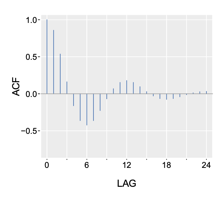
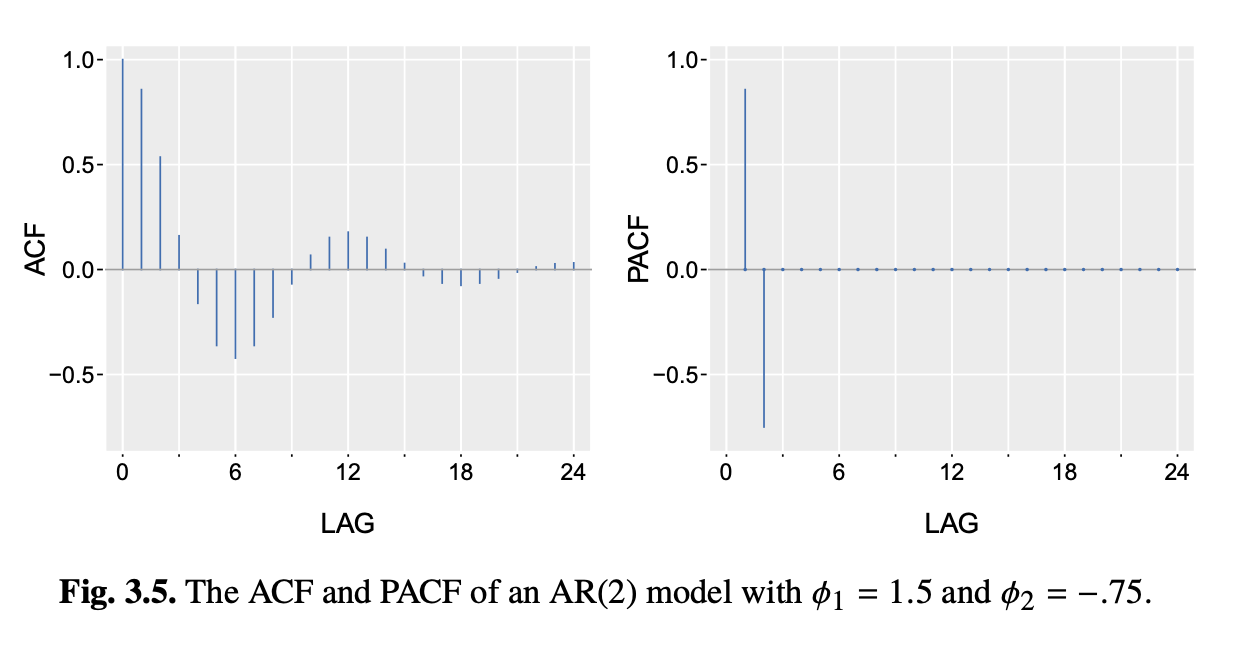
The ACF oscillates and decays gradually — it tails off. The PACF has two non-zero spikes and is essentially zero from lag 3 on — it cuts off after lag 2. That's exactly the AR(2) row of the table above.

Worked example: sunspot numbers

The classic sunspot record — the built-in statsmodels series of yearly sunspot numbers, 1700 to 2008 — has a well-known, roughly 11-year cycle. Before looking at its ACF and PACF, it's worth guessing: is the autocorrelation slowly decaying, oscillating, or does it cut off sharply? Would you expect an AR, MA, or ARMA structure, and roughly how many parameters?

What the data show: the ACF decays slowly and oscillates — the 11-year cycle shows up as a damped sinusoid in the correlogram — while the PACF drops sharply after lag 2. That combination is exactly the AR(2) signature from the diagnostic table. The striking part is that just two coefficients are enough to generate this quasi-periodic behaviour.

Fitting AR(2) by maximum likelihood gives

\[\hat\phi_1 = 1.3906, \qquad \hat\phi_2 = -0.6886,\]

with a fitted mean level of about \(49.75\). The characteristic roots of the fitted AR polynomial form a complex-conjugate pair, \(0.6953 \pm 0.4529i\), with modulus \(0.8298\) — close enough to 1 that the implied oscillation is only lightly damped, which is why an 11-year cycle originally estimated from an 11-year physical process persists throughout a three-century record rather than dying out. The angle of that root gives an implied period of about \(10.9\) years, matching the sunspot cycle's actual period of roughly 11 years closely.

Having fit the model, the next question is whether AR(2) is enough: check the residuals. If the model has captured all the correlation structure, the residual ACF and PACF should be essentially zero at every lag but 0. For sunspots, the AR(2) residuals are close to white noise — though not quite: the periodicity is not entirely removed. Even so, this is a good example of the general signature of an AR process: an ACF that decays gradually, driven by a PACF that cuts off after a small number of lags.

Worked example: gas prices

Not every series is this clean. The second example is the FRED series GASREGW, the weekly US average price of regular gasoline. Gas prices show strong persistence, but they also react to shocks — supply disruptions, policy changes — that create short-lived deviations, a structure that suggests both AR and MA behaviour might be at play.

The raw series has 1,853 weekly observations (mean $2.26, standard deviation $0.95). The lecture works with two versions of it: the level series, and its log first difference — the week-to-week growth rate.

Before looking, it's worth predicting: would you expect the ACF to decay faster or slower than the sunspot series? Will the PACF cut off as cleanly?

What the data show: the ACF of the level series decays very slowly — high persistence, close to a unit root — while its PACF has a strong spike at lag 1, a smaller one at lag 2, and then starts to cut off. Differencing removes most of that persistence: the ACF of the log-differenced series falls off noticeably faster.

From there the notebook works through the sequence a modeller would try on the differenced series: AR(1), AR(2) and AR(4); then MA(1), MA(2) and MA(4) as an alternative; then an ARMA(1,1) combining one AR term and one MA term. (Which of these looked cleanest by eye is left as a live class discussion rather than written down — the notebook only records the fits and the residual plots, not a stated verdict.)

To settle the comparison quantitatively, the models are instead compared out-of-sample: fit on all but the most recent part of the series, forecast forward, and compare root-mean-square forecast error. There's a wrinkle worth noticing in how the holdout is built: the code's comment says the last "3 years" are held out, but the line that would convert weeks to years (t = 3 #*52) has the multiplication commented out — so the actual test set is just the last 3 weekly observations out of 1,852, not three years of them. With that caveat, the reported forecast RMSE on the log-differenced series is:

Model	RMSE
AR(1)	0.02041
AR(2)	0.02074
AR(3)	0.02322
AR(4)	0.02445
ARMA(1,1)	0.02099
ARMA(2,1)	0.02565
ARMA(3,1)	0.02379

(train: 1,849 observations; test: 3.)

Exercises

From the lecture's own notebook (Lecture 18); restated here, not answered.

1. Using the RMSE table above: does adding more AR lags keep helping, or does performance get worse past some point? What does that suggest about how many AR terms the gas-price growth rate actually needs — and how much should you trust a comparison built on a 3-observation test set?
2. How does ARMA(1,1) compare to the pure AR models in the table? Is the single MA term buying anything?
3. Conceptually, rather than just from the numbers: why might a series like gas-price growth have both autoregressive and moving-average structure, rather than being cleanly one or the other?

Sources

• ARMA recap, causality/invertibility statements, ACF-vs-PACF motivation, the general partial correlation formula, and the ACF/PACF diagnostic table: 18_arima_models_notes.md (Lecture 18 notes, Berkeley Stat 153/248, spring 2026).
• The two illustrative AR(2) figures (\(\phi_1=1.5,\phi_2=-0.75\)) are images linked from that same notes file.
• The sunspot AR(2) worked example (data, prediction prompt, fit, characteristic roots, residual check): Lecture18/01-stat-153-248---lecture-18.md and Lecture18/02-what-do-we-see.md, converted from the lecture's notebook Lecture18.ipynb.
• The gas-price example (FRED series GASREGW), the AR/MA/ARMA comparison, the forecasting RMSE table, and the closing discussion questions used above as exercises: also Lecture18/02-what-do-we-see.md.
• Referred to but not supplied: Shumway & Stoffer, Time Series Analysis and Its Applications, Chapter 3 and Appendix B2 (causality/invertibility proofs) and §3.3.2 (PACF derivation); the plotted figures for the sunspot and gas-price analyses themselves, which appear in the converted notebook only as "figure omitted" placeholders.
• The notebook's introduction also names a third motivating dataset, heart rate variability (HRV), which is not present in the supplied material and so is not covered here.
• No transcript and no separate problem set were supplied for this lecture.

---

← 15. Autoregressive Moving Average Models · Contents · 17. Fitting and Diagnosing ARIMA Models →